Parameters for Graphs

A wide variety of parameters can be set that influence the look of graphs. As explained in the introductory entry, many of these parameters can be changed 'ad hoc', i.e., with respect to a single element of a single graph; yet, they also can be set prior to creating a graph and remain valid until further change (or set back to the default value). This is the way parameter settings are presented here.

Again, this entry is far from complete. See ?par for an overview of parameters. The command

par()

will yield a list of current parameter settings. Of course, you may store this list to an R object via, e.g., pp <- par(). For instance, before tinkering with parameters you may wish to store the default values with some such commmand (some users seem to prefer pp <- par(no.readonly = T), with the additional option implying that only those parameters are stored that can be changed) and restore them any time you want with, e.g., par(pp).

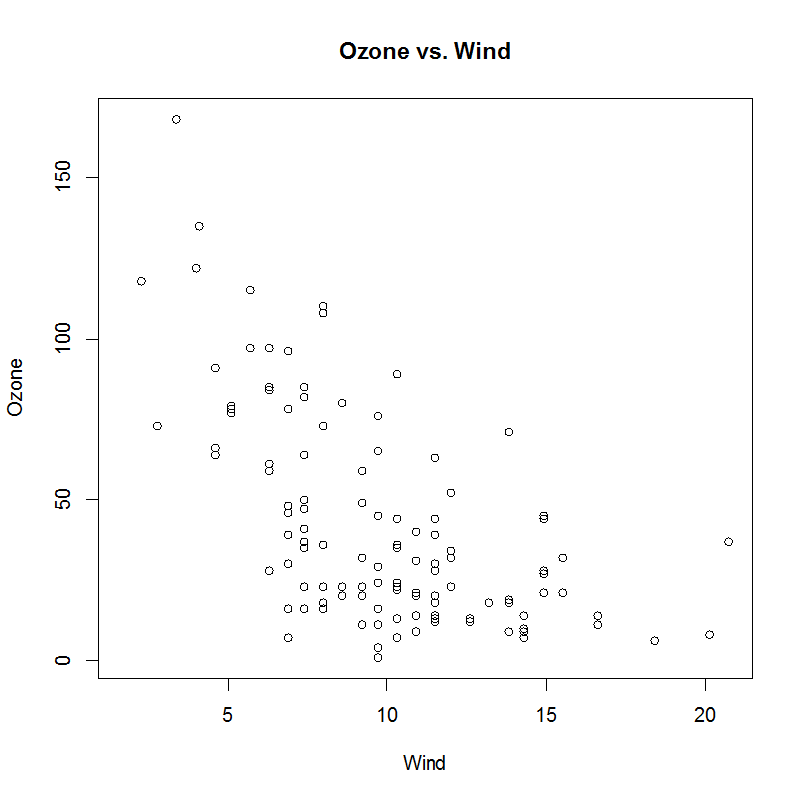
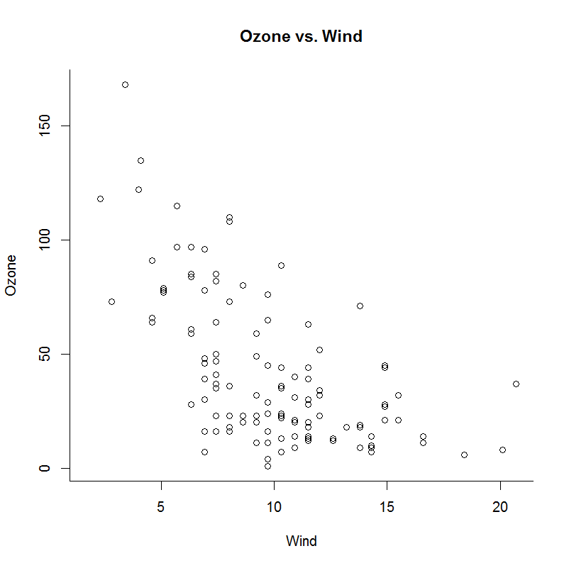
The graphs that follow use the "air quality" data that come with R. The examples may easily be reproduced by first attaching the data (attach(airquality)) and, after setting the parameters, creating the graph with plot(Wind,Ozone, main="Ozone vs. Wind").

Margins

Margins around the plot

There are two ways to influence the margins around the plot. The first gives the margins in inches, as in

par(mai = c(0.5, 0.5, 0.5, 0.5))

with the numbers referring to the bottom, left, top, and right margins (the default values are 1.02, 0.82, 0.82, and 0.42). The second gives the margins in terms of "lines" (i.e., lines of text), as in

par(mar = c(3, 3, 3, 3))

(the default values are 5.1, 4.1, 4.1 and 2.1). Note that expert users would have written these commands as par(mai=rep(0.5,4)) and par(mai=rep(3,4)), but of course this works only because in my examples all four margins are the same, which in many instances will not be the case.

Why change the margins? Normally, the best thing is to leave them as they are. However, occasionally the need to change them may arise. For instance, when combining several graphs, reducing the margins may be helpful to better fill the "cells" of the final plot. Or an axis label may require more space than is normally available. Or ... (make your own list here).

Size of plotting elements

Overall size

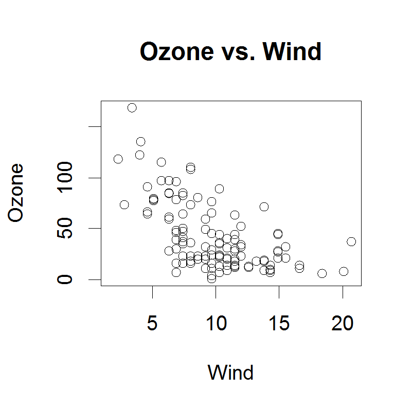
The size of plotting elements (symbols, text, or even axes) can be manipulated by cex, the default value of which is 1. Thus, changing the parameter via, e.g.

par(cex = 1.2)

will increase all the elements in the plot by a factor of 20 per cent. The two plots that follow compare the default settings with cex=2, just for the sake of demonstration.

Graph with cex=default Graph with cex=2

Single elements

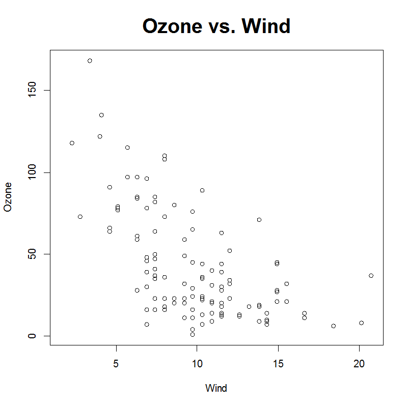
As the example above demonstrates, simply changing cex is not a good idea in most circumstances. Usually, you will want to change single elements. The next example demonstrates the effect of

par(cex.main = 2)

i.e., of changing the size of the title, on the left, and of

par(cex.main = 2, cex.axis = 0.5, cex.lab=2)

i.e., of changing the size of the title, the axis annotion, and the axis labels on the right. The values in the latter example were chosen for demonstration purposes; in no way these settings are recommended!

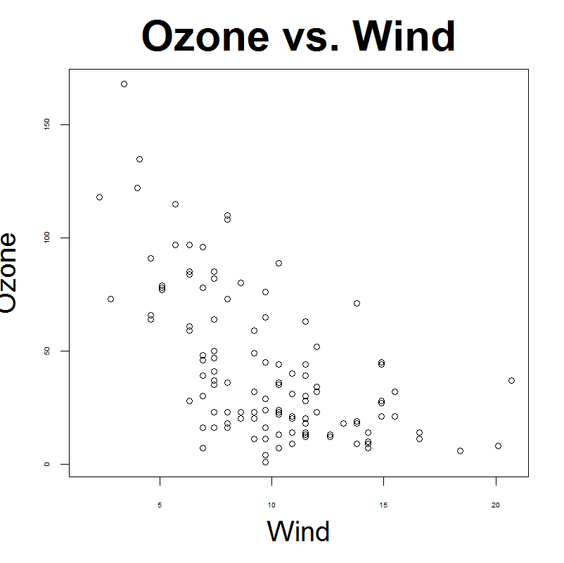
Graph with cex.main=2 Graph with several elements changed

Note particularly that as a result of the axis label magnification, the y axis label (Ozone) is "cut off" at the top in the graph on the right hand side (this is not an effect of the web display; it's in the original graph). This is a case where you might want to increase the left margin, as in par(mai=c(1,1.5,1,1)).

Other elements

The box around the plot

Normally, a box surrounds each plot. You may change this box with the bty (box type) parameter, as in:

par(bty = "l")

Note that the parameter for bty is the letter "l", not the number one. Actually, it would be even better if the parameter were "L", as this would indicate what happens: The box is drawn as an "L", i.e., only on the bottom and the left side.

Other parameters are "7", "c", "u", or "], with "o" as the default, and "n" for no box at all. The following examples shows the effect of "n" (left) and "l" (right).

Graph with bty=n Graph with bty=l