Exploratory Data Analysis

I present only the two most popular graphs, namely, stem-and-leaf displays and box-and-whisker plots, aka boxplots.

Stem-and-leaf displays

Stem-and-leaf displays are a good way of looking at the shape of your data. They are apt particularly for smaller data sets.

Unsurprisingly, the command is stem, as in

stem(mydata$quality)

Stem and leaf displays, as implemented in R, are not meant for huge data sets. In other words, there is no procedure to combine several values into a single leaf. A few options give you some control over the display of the graph, though.

stem(mydata$quality, width=120, scale = 2)

will increase the standard width of 80 characters per line to 120 and in addition try to spread out the graph by producing more stems. (The latter option was used in the display on the left.)

13 | 3
14 | 16
15 | 89
16 | 0679
17 | 123677
18 | 0134
19 | 01222566
20 | 1279
21 | 3799
22 | 022489
23 | 5
24 | 57
25 | 3
26 | 014

Box-and-Whisker Plots

Colloquially known as "box plot" (or "boxplot"), this is one of the most well-known pieces from John W. Tukey's impressive toolbox. It is used to get a rough idea of the distribution of a variable, either "as is" (univariate case) or (perhaps more frequently) to compare the distribution over groups (bivariate case).

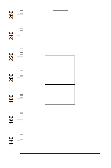
Univariate boxplot

A boxplot like the one shown here can be obtained as follows:

boxplot(mydata$quality)

The small ticks on inner side of the y axis represent the data points. They were created by adding the following command (note that this is not an option to the boxplot command; it is a new command that is entered after the plot has been created):

rug(mydata$quality, side=2)

Note that rug is not specific to the boxplot; it can be added to any plot, whether it's meaningful or not. The side option controls, obviously, on which side the rug is plotted (the default = 1, at the bottom).

The boxplot command has some options of its own, some of which will be treated below.

Boxplots by group

The basic version is

boxplot(metricvar ~ groupvar, data=name-of-data-object)

Note that what I have termed "groupvar" here need not be a factor; it may be a numeric variable as well, the different values of which will treated as representing different groups.

Elements of the boxplot

A variety of options is available; here are a few you might wish to consider. In these examples, options that refer to the boxes presuppose that three boxes are present.

`notch=TRUE`	draw boxes with notches
`col=c("grey60", "grey40", "grey20")`	colors (in this examples, greyscales) to distinguish the boxes
`border=c("blue", "burleywood4", "red")`	colors for the borders of the boxes
`names=c("Manual", "Clerical", "Service")`	labels for the boxes (if those created automatically do not please you)

Note that the notches describe an approximate confidence interval for the median. More about colours can be found here.

Lattice and ggplot2 versions

The ggplot2 library offers its own version of the boxplot.

The lattice library includes a procedure bwplot which perhaps will be outlined in more detail later.