Results of MCMC Models via Coda

As yet, this site says nothing about MCMC. I just want to give some illustrations of the output from the Coda package.

My example shows three parameters from a more complex model. The parameters were chosen such as to demonstrate "sucessful" and "not so successful" estimation results. The example is based on 50,000 iterations, of which 25,000 were discarded as burn-in, and on two chains.

I have used OpenBUGS (via R2OpenBUGS). Note that to use the Coda package, you have to invoke R2OpenBUGS with option codaPkg=T. Also, you have to "convert" the results (assumed to be stored in myModel) for further processing as follows:

myModel.coda <- read.bugs(myModel)

Numeric output

Normally, we will first want to see the parameter estimates plus credible intervals (via quantiles):

summary(myModel.coda)

A numeric measure for convergence of the chains (it should be close to unity) is requested via

gelman.diag(myModel.coda)

Finally, we may be interested in the effective sample size:

effectiveSize(myModel.coda)

In the case under investigation, we note that the Gelman statistic for the troubling parameter is 1.01, which is not too troubling. However, the effective sample size is 28 only. This is a cause for some concern.

There is a lot of other things that can be done with MCMC-output. First, you can get a rather close look at the structure of the output with head(myModel.coda). You may also extract parts of the output. For instance,

c2.10

will extract the first 100 iterations of column 10 in chain 2.

xy plot

This plot shows whether the two chains converged to common parameters. Assuming that the parameters of interest are stored in colums 2 to 4, we write:

xyplot(myModel.coda[,2:4])

Coda - plot

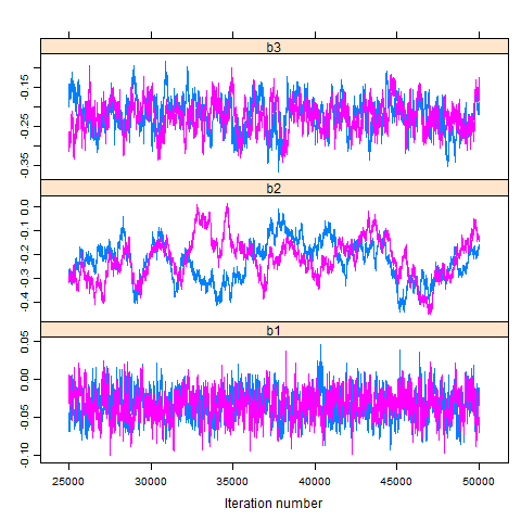
The plots show a lack of convergence in the case of parameter b2, except for the last few thousand iterations. That is, while concergence has eventually been reached, the entire chain of 25,000 iterations contains much noise.

Trace and density

Both are available as separate plot, but they are available together via the plot method:

plot(myModel.coda[,2:4])

Coda - xyplot

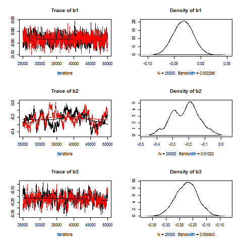
Again, we note the lack of convergence in the case of b2. Also, the density distribution is rather irregular, again a bad sign.

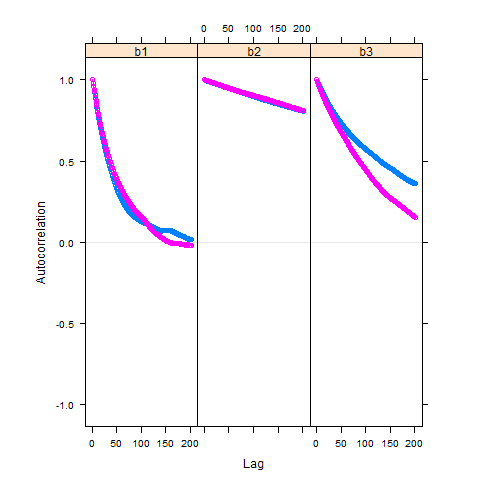
Autocorrelation

Autocorrelation is high for all three parameters, but it is a huge problem for parameter b2:

acfplot(myModel.coda[,2:4], lag.max=200)

Coda - acfplot

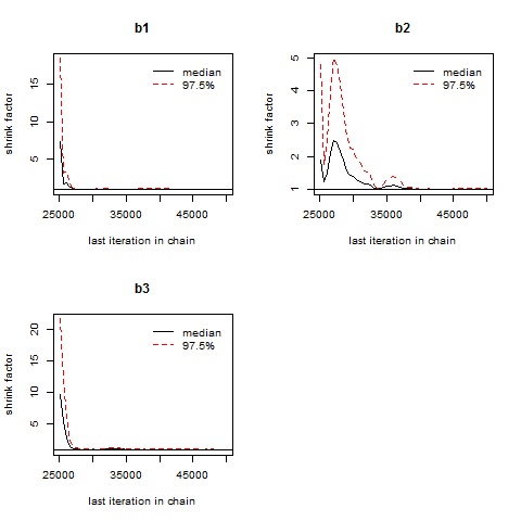
Gelman plot

This plot shows again that estimates for b2 cannot be trusted, since only the last 10,000 iterations have brought about satisfactory results.

gelman.plot(myModel.coda[,2:4], lag.max=200)

Coda - Gelman plot