Three-dimensional Graphs

As usual, R offers an amazing number of possibilities. This section deals only with a simple surface plot that uses the standard function persp; note also the more traditional contour plots and image. Other graphs are offered in the lattice package (try wireframe for surface plots), or in package plot3D and a number of other (often more specialized) packages.

Explaining persp()

The most important thing is to understand how to organize the input for such a graph. What you need is:

A vector with n values for the x axis,
another vector with m values for the y axis, and
an n × m matrix with the values that correspond to all combinations of x and y (even though missing values, i.e. NAs, are permitted).

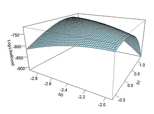
Luckily, with R this can be obtained quite easily (once you have found out how it is to be done). Look at the following example: I want to show the Log-likelihood of a two-parameter logistic regression modell (a constant and one additional coefficient). The constant was -2.4373 and the coefficient .349, and the data consisted of 2.307 cases for which I know the values of the dependent variable (0 or 1) and of the independent variables (which was also a dichotomous variable with values 0 and 1).

First, we must create a sequence of values in the region of the constant and the regression coefficient:

x <- seq((-2.4373 - .5),(-2.4373 + .5), .02)
y <- seq((.349 - 1),(.349 + 1), .05)

Next, a function is needed that tells R what to do with the values of x and y. In my case, this is a very simple, even though a bit long, expression:

f <- function(x, y) {
1087*log(1-(exp(x)/(1+exp(x)))) +
95*log(exp(x)/(1+exp(x))) +
1001*log(1-(exp(x+y)/(1+exp(x+y)))) +
124*log(exp(x+y)/(1+exp(x+y)))
}

Finally, we require the outer product of x and y:

k <- outer(x, y, f)

Now, we've got all we need:

persp(x, y, k, theta = 30, phi = 20, expand = 0.5, col = "lightblue",
ticktype = "detailed", xlab = "b0", ylab = "b1", zlab = "Log-Likelihood" )

The result looks as follows:

Drei-dimensionaler Plot einer Maximum Likelihood-Funktion